
The Laboratoire d'Astrophysique de Bordeaux
(LAB) participates in the International
VLBI Service for Geodesy and Astrometry (IVS) as an Analysis Center. One of the goals of the IVS is to
maintain the “International Celestial Reference Frame” (ICRF). The ICRF is a catalog of VLBI
positions of several thousands extragalactic radio sources which are used as references in
the sky.
Although these sources show very compact radio emission, they are however not prefect fiducial markers on the sky. They can exhibit structure on VLBI scales, and their position can fluctuate over time. For this reason, all ICRF sources are monitored on a regular basis in order to track variations in position and structure.
In this context, one of the contributions of the LAB consists in producing VLBI images of these extragalactic radio sources and to assess their structure.
Such images, along with additional products (structure correction maps, visibility maps, flux density values, etc.), are provided to the community through the Bordeaux VLBI Image Database (BVID).
More details
-
The International VLBI Service for Geodesy and Astrometry (IVS)
The IVS is an international collaboration of organizations which support Very Long Baseline Interferometry (VLBI).
The goals of IVS are:
- To provide a service to support geodetic, geophysical and astrometric research and operational activities.
- To interact with the community of users of VLBI products and to integrate VLBI into a global Earth observing system.
- To promote research and development activities in all aspects of the geodetic and astrometric VLBI technique.
Further information about the IVS and its activities may be found at https://ivscc.gsfc.nasa.gov/.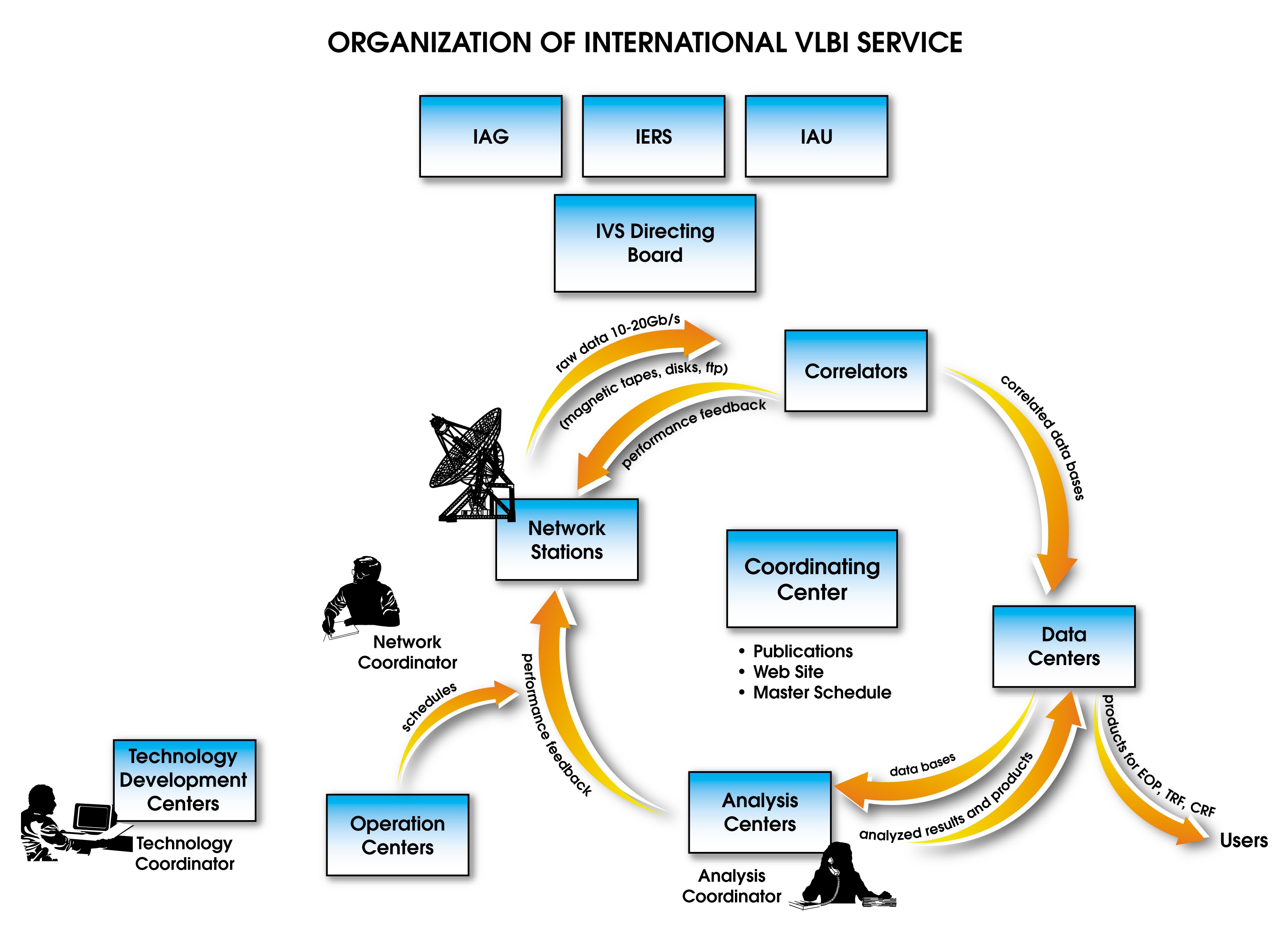 The organization of the IVS (Credit: IVS)
-
The International Celestial Reference Frame (ICRF)
The ICRF is the realization of the International Celestial Reference System (ICRS) at radio wavelengths, and is the fundamental celestial reference frame adopted by the International Astronomical Union (IAU). The current version of the ICRF is the ICRF-3, which comprises VLBI positions for 4536 extragalactic radio sources, including 303 defining sources, i.e. sources that set the direction of the frame axes (see figure below).The position accuracy, for the majority of the ICRF-3 sources, is well below the sub-milliarcsecond level (i.e. a few nanoradians) with a noise floor of 0.03 mas. This accuracy depends on first hand on the number of observations but also on the positional stability and the compactness of the sources. Point-like sources with no positional variation in time are ideal sources for building such a reference frame. Unfortunately, very few extragalactic sources (and therefore ICRF-3 sources) are truly point-like. Most of them exhibit structures on VLBI scales, and those structures can also fluctuate over time, as show in the images below.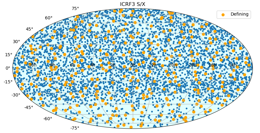 Distribution on the sky of the 4536 sources of the ICRF-3 (Credit: IERS ICRS Center/Paris Observatory)
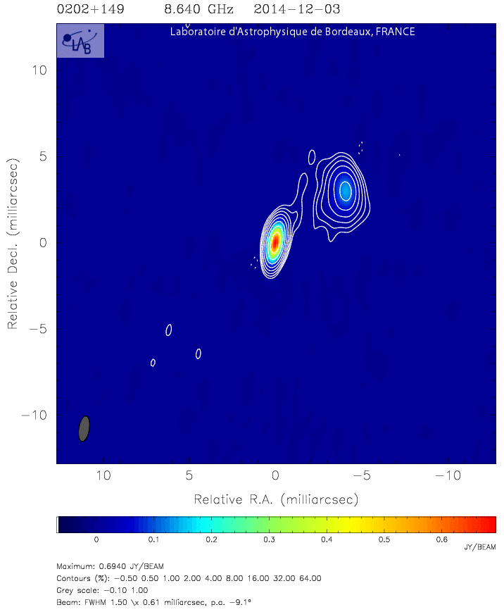
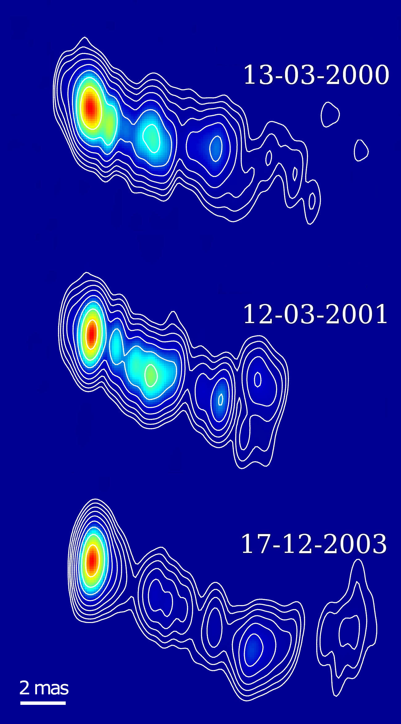
Left panel: Example of a source with a non point-like structure. Right panel: Case of a source with a structure evolving with time.
(Credit: BVID)
The images made available throught the Bordeaux VLBI Image Database (BVID) allows one to assess the compactness and to monitor the structural evolution of the reference frame sources, which is essential for maintaining and improving the frame. Besides the astrometric applications, the BVID images are also useful for astrophysical studies, i.e. for investigating source morphology and superluminal motions in extragalactic radio sources.
The BVID is complementary to the Fondamental Reference Image Data Archive (FRIDA) maintained at the United States Naval Observatory (USNO).
Further information about the ICRS and the ICRF may be found at https://aa.usno.navy.mil/faq/ICRS_doc.
-
The International Terrestrial Reference Frame (ITRF) and the Earth Orientation
Parameters (EOP)
In addition to the positions of the radio sources, the VLBI technique also permits to determine the positions of the radiotelescopes on Earth and the orientation of the Earth.
The positions of the radiotelescopes contribute to the “International Terrestrial Reference Frame” (ITRF) while the monitoring of the Earth orientation allows one to track irregularities in its rotation. The orientation of the Earth is described through five parameters (EOPs), which are the following:
— the coordinates of the pole (x, y), which point to the position of the Earth's rotation axis with respect to the crust,
— the Universal Time (UT1-UTC), which describes the rotation of the Earth around that axis,
— the celestial pole offsets (dX, dY), which charaterize the direction of the Earth rotation axis relative to the celestial frame (precession and nutation motion).
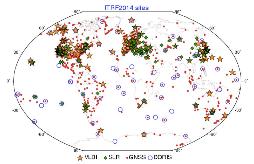
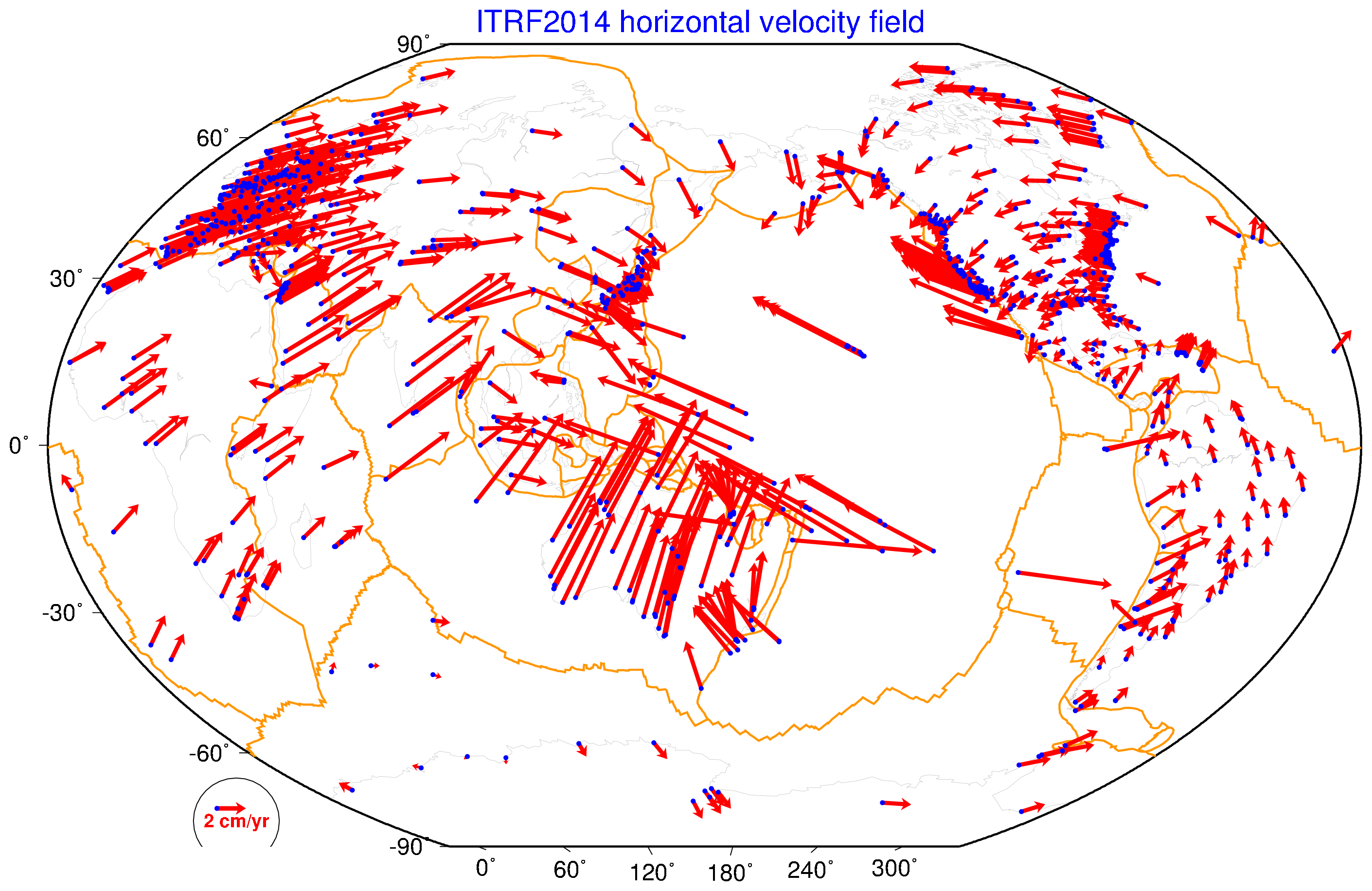
Left panel: Positions of the stations in the ITRF2014 Right panel: Velocities of the stations in the ITRF2014.
(Credit: Altamimi et al., 2016)
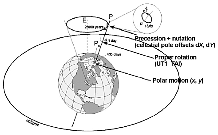
The Earth Orientation Parameters EOPs (Credit: Vondrák 2009)
For further details about the ITRF, please see the dedicated website at https://itrf.ign.fr/en/homepage. For the EOPs, go to https://hpiers.obspm.fr/eop-pc/index.php.
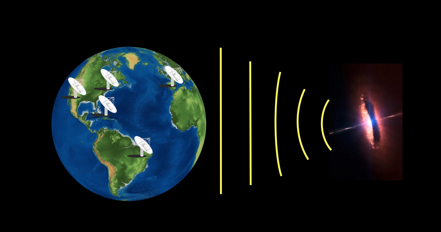 Illustration of the VLBI concept (Credit: A. Collioud / BVID)
With the Very Long Baseline Interferometry (VLBI), the distance between radiotelescopes is typically intercontinental and extends to several thousands of kilometers. This makes VLBI a unique technique to image the observed sources in their finest details and to position them in the sky ultra-accurately.
More details
-
The principle of VLBI
Mathematically, the maximum resolution (the size of the smallest details that can be observed) of an interferometer depends on the wavelength λ and the distance B between the two most-separated antennas (the maximum baseline length), and is equal to ~ 1.22 λ/B.
Some interferometers are comprised of physically connected antennas, i.e. linked by cables, optical fibers or radio links. In this case, the distance between antennas is limited to a few dozens kilometers and the correlation is done in real-time in a nearby correlator. In contrast, the VLBI arrays consist of independant antennas. The longest possible VLBI baseline corresponds to the diameter of the Earth (~12000 km), and the highest resolution is at or below the milliarcsecond level at centimeter wavelengths. For example, for λ = 4 cm (X-band) and B = 12 000 km, the resolution is about 0.8 milliarcsecond. This corresponds to a 2 euro coin seen at a distance of 6700 km, i.e. roughly the distance between Paris (France) and Chicago (USA).
The principle of the VLBI technique can be described as follows (see also the figure above):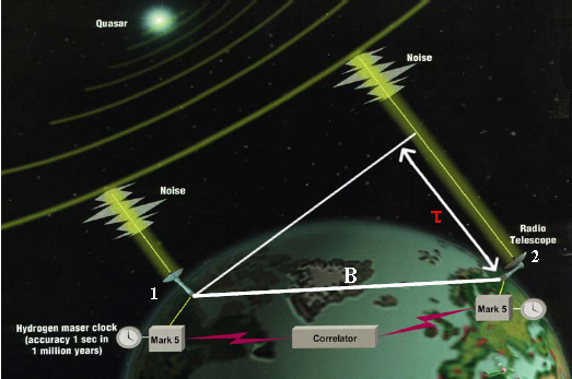 The principle of the VLBI technique (Credit: NASA/GSFC)
- A very distant radio source emits radio waves, which are received by two stations (1 and 2) on Earth, forming the baseline B. The radio signal is received at the station 2 with a time delay τ, which depends mostly on the geomety of the baseline relative to the source direction.
- Each station records the radio signal on disks, along with precise timing information, usually delivered by a local hydrogen maser.
- At the end of the observation, the disks are sent to a remote correlator.
- At the correlator, the two signals are read, “played back” and multiplied together (correlated) in order to generate interferometric patterns containing information about the radiosource (direction on the sky, brightness distribution), the baseline vector and the Earth's orientation.
The radio signals can also be directly transfered from each station to the correlator through high-speed networks, and correlated in real-time: this is called “e-VLBI” (for electronic-VLBI).
-
The VLBI networks and observing sessions
Making VLBI observations requires coordination between antennas located all around the world, which by nature, implies international cooperation. Over the years, several arrays of antennas have developped. At present, the three main VLBI arrays are:
- The European VLBI Network (EVN) mostly in Europe, but also with antennas in Asia, South Africa and Porto-Rico,
- The Very Long Baseline Array (VLBA) in the USA,
- The IVS network, which covers all continents.

The IVS Network (Credit: IVS)
Most of the VLBI images available in the BVID were produced from the data of the RDV sessions.
The primary observable for geodesy and astrometry is the difference in the time of arrival of the radio source signal at two antennas. This time difference is called time delay or more simply delay (τ). This delay depends mostly on the relative geometry between the radio source direction in the sky and the baseline vector formed by the two antennas. It also depends to a lesser extent on other contributions like the atmosphere, the instrumental errors, etc.
By measuring and modeling the delay for each baseline of the network, one can precisely infer the position of the observed radio sources in the sky, the position of the antennas on Earth, and the orientation of the Earth.

The VLBI delay (Credit: Teke et al., 2012)
More details
The delay τ is dominated by a geometric component
(see the illustration in the VLBI technique section). The other
contributions originate from:
Proper modeling of each of these components allows one to precisely estimate the radio source positions, the antenna positions and the Earth's Orientation Parameters (polar motion, Earth's rotation, precession-nutation).
The most accurate VLBI observable is the phase delay which is defined as:
τφ = φ / ω
where φ is the fringe phase and ω the angular frequency (ω= 2πν, where ν is the frequency).
The phase delay however is ambiguous since the phase is only known modulo 2π. On the other hand, the group delay which is the derivative of the phase delay with respect to the angular frequency (∂φ / ∂ω) does not suffer from such ambiguities, although less accurate. It is the primary observable used for geodesy and astrometry.
In practice, the group delay (or bandwidth synthesis delay) is determined by fitting a straight line to the phases measured at several discrete frequencies, as shown in the figure below. The RDV sessions usually comprise four such frequencies at X band (e.g. 8366, 8446, 8806 and 8926 MHz) and another four frequencies at S band (e.g. 2241, 2271, 2361 and 2381 MHz).

Fit of the measured phases at 8 discrete frequencies at X band to determine the group delay (Credit: Charlot 2007)
- the atmosphere, i.e. the troposphere (comprising a dry and a wet component) and the ionosphere (delay caused by the total electronic content) ; the latter can be removed by combination of simultaneous observations at X-band and S-band,
- instrumental effects: clock offsets and instabilities, delay in cables and electronic components, etc.,
- relativistic effects,
- source structure effects (see the structure correction maps section).
Proper modeling of each of these components allows one to precisely estimate the radio source positions, the antenna positions and the Earth's Orientation Parameters (polar motion, Earth's rotation, precession-nutation).
The most accurate VLBI observable is the phase delay which is defined as:
τφ = φ / ω
where φ is the fringe phase and ω the angular frequency (ω= 2πν, where ν is the frequency).
The phase delay however is ambiguous since the phase is only known modulo 2π. On the other hand, the group delay which is the derivative of the phase delay with respect to the angular frequency (∂φ / ∂ω) does not suffer from such ambiguities, although less accurate. It is the primary observable used for geodesy and astrometry.
In practice, the group delay (or bandwidth synthesis delay) is determined by fitting a straight line to the phases measured at several discrete frequencies, as shown in the figure below. The RDV sessions usually comprise four such frequencies at X band (e.g. 8366, 8446, 8806 and 8926 MHz) and another four frequencies at S band (e.g. 2241, 2271, 2361 and 2381 MHz).
Fit of the measured phases at 8 discrete frequencies at X band to determine the group delay (Credit: Charlot 2007)
The two observables used for imaging are the amplitude and phase that result from the correlation process for a given observation. Amplitude and phase form a quantity called complex visibility which can be mathematically related to the brightness distribution of the source. Using such measurements acquired over different times and baselines, it is then possible to reconstruct an image of the radio source.
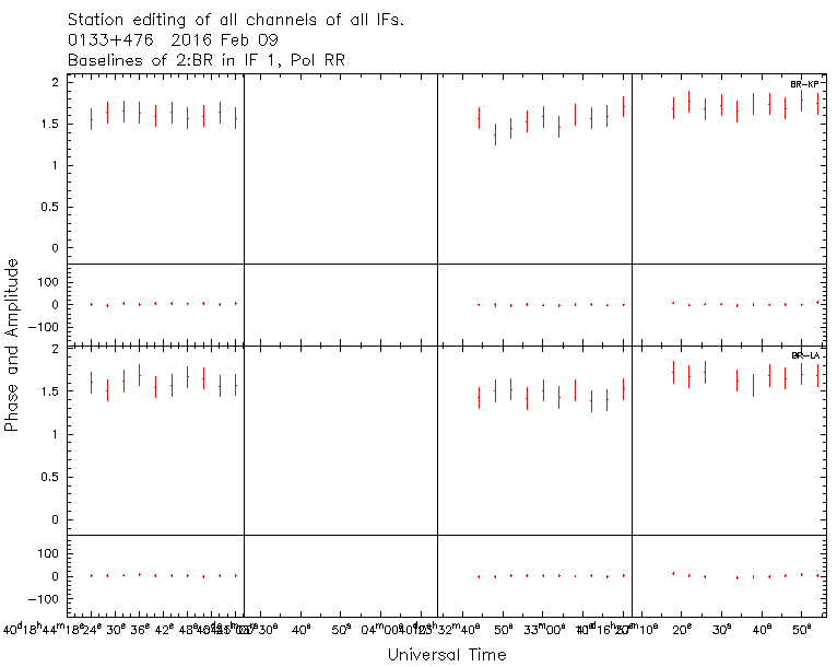
VLBI amplitudes and phases for two different baselines (Credit: BVID)
More details
Mathematically, it is possible to demonstrate that the complex visibility (quantity
measured by an interformeter) is the 2-dimension Fourier transform of the spatial
brightness distribution of the source. This is the Van Cittert-Zernike
theorem. By using an inverse Fourier transform, one can then, in theory, reconstruct
the image of the radio source from the complex visibility measurements.
Unfortunately, the VLBI technique usually provides a poorly-sampled Fourier plane, also known as the (u,v) plane. Due to the sparseness of the network, the visibility is measured only at a limited number of points of the (u,v) plane ,which correspond to the projection of the observing baselines on the sky, and has undefined values elsewhere. In such a case, the reconstruction process (i.e. the inverse Fourier transform) leads to an incomplete and distorted image: the dirty map. This dirty map is in fact the convolution of the source brightness distribution with the dirty beam, which is the Fourier transform of the sampling function (i.e. the representation of the network in the Fourier domain). This is summarized in the figure below.
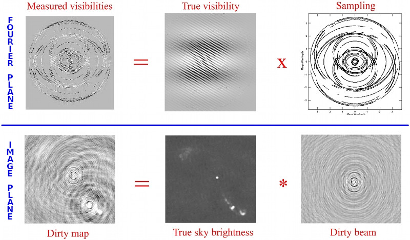
Upper panel: Imaging in the Fourier plane — the visibilities measured by the interferometer are obtained by multiplying the true visibility distribution by the sampling function.
Lower panel: Imaging in the image plane — the dirty map is the convolution of the source brightness distribution by the dirty beam.
Upper and lower panels are related by a direct (or inverse) Fourier transform.
(Adapted from Garrington 2007)
In order to “interpolate” the complex visibility values at the unsampled
points of the (u,v)-plane and reconstruct a realistic image, one can use non-linear deconvolution methods, such as
the CLEAN algorithm or the Maximum Entropy Method (MEM) incorporating also some physical
assumptions about the image (e.g. the sky has always positive brightness, is mostly empty, etc.).
Unfortunately, the VLBI technique usually provides a poorly-sampled Fourier plane, also known as the (u,v) plane. Due to the sparseness of the network, the visibility is measured only at a limited number of points of the (u,v) plane ,which correspond to the projection of the observing baselines on the sky, and has undefined values elsewhere. In such a case, the reconstruction process (i.e. the inverse Fourier transform) leads to an incomplete and distorted image: the dirty map. This dirty map is in fact the convolution of the source brightness distribution with the dirty beam, which is the Fourier transform of the sampling function (i.e. the representation of the network in the Fourier domain). This is summarized in the figure below.
Upper panel: Imaging in the Fourier plane — the visibilities measured by the interferometer are obtained by multiplying the true visibility distribution by the sampling function.
Lower panel: Imaging in the image plane — the dirty map is the convolution of the source brightness distribution by the dirty beam.
Upper and lower panels are related by a direct (or inverse) Fourier transform.
(Adapted from Garrington 2007)
The celestial objects observed with the VLBI technique are usually very bright and distant active galaxies. These objects possess a tremendous energy which originates from the accretion of dust and gas by a supermassive black hole located in the innermost region of the galaxy. This region is called the Active Galactic Nucleus (AGN). The radio emission is of synchrotron origin and comes from relativistic jets in the inner AGN part.

Artist's impression of an AGN (Credit: ESO/M.Kornmesser)
More details
Active galaxies come with several
“species”: radiogalaxies, quasars, Seyfert galaxies, BL Lac, Blazars, etc., which have each specific properties.
In all, the different “species” may in fact be related to a single type of physical object observed from different angles (see figure below); this model is called the unified model of AGN. Further details about AGN may be found in the review: Padovani et al. 2017, Astron Astrophys Rev, 25, 2 (Pdf file )
)
In all, the different “species” may in fact be related to a single type of physical object observed from different angles (see figure below); this model is called the unified model of AGN. Further details about AGN may be found in the review: Padovani et al. 2017, Astron Astrophys Rev, 25, 2 (Pdf file
 )
)
VLBI images reveal the structure (i.e. the brightness distribution) of the extragalactic radio sources on milliarcsecond scales. Such structures can vary in both time and frequency, and set limits on the accuracy of source positions determined with VLBI astrometry unless their effects are accounted for.
Images available in the BVID were produced from VLBI observations at S-band (2 GHz, λ= 13 cm) and X-band (8 GHz, λ=4 cm). For some sources, images are also available at K-band (24 GHz) and Q-band (43 GHz).

Mosaic of VLBI images displaying various source morphologies (Credit: BVID)
More details
At the Bordeaux Analysis Center, VLBI images are typically produced following two steps.
-
First, the correlated data are calibrated using the Astronomical Image Processing System (AIPS)
software, following the reduction path summarized below:
- Bad data are removed using flagging information recorded during the session at each station (antenna not yet on source, channel error, etc.).
- Initial amplitude calibration is applied using the measured system temperatures and the gain curve provided for each station.
- Fringe fitting is accomplished to remove the residuals remaining in the delay (and time derivatives of delay) after correlation due to the atmosphere, clocks offsets, errors in the position of the stations, etc. The fringe-fitting process consists in searching the maximum of the fringe amplitude over the delay and delay rate parameter space. A valid detection is obtained if the maximum amplitude is greater than a specified level (defined by a Signal to Noise Ratio value).
- A refined amplitude calibration is then applied, using gain correction factors determined following model-fitting of one or several calibration sources (i.e. strong and point-like sources) observed during the same session. The gain correction factors are determined by fitting structure models to the measured visibilities of the calibration sources and then applied to all sources observed in the session.
- Finally, the calibrated data are exported as FITS files (one FITS file per source).

The AIPS data processing pipeline (Credit: A. Collioud / BVID) -
The FITS files are then processed to image each source by using the Caltech VLBI imaging
software Difmap in automatic mode (Shepherd et al. 1995).
The procedure is based on the hybrid-mapping technique (Readhead & Wilkinson 1978)
with a point-source model at start. Visibilities are self-calibrated (only the phases at first,
and then the phases and amplitudes in subsequent rounds), Fourier-inverted, and CLEANed. Uniform weighting and,
after several iterations, natural weighting, are successively applied to derive the
final VLBI image.
The VLBI image is the convolution of a model of the source (i.e. a set of CLEAN components) with the CLEAN beam (i.e. an elliptical gaussian fitted to the central lobe of the dirty beam).

Example of processing with Difmap (Credit: A. Collioud / BVID).
Left panel: A residual map
Right panel: A CLEAN map showing the CLEAN components of the source model

Structure correction map (Credit: BVID)
The structure index is derived from the median value of the structural delay values for all possible Earth-based baselines. The structure index indicates the magnitude of the structure of the source: the smaller the structure index value, the lower the effect of the source structure.
More details
The structure correction maps display the magnitude of intrinsic source
structure effects on the basic quantity measured in astrometric/geodetic VLBI, i.e. the
bandwidth synthesis delays, as a function of interferometer resolution.
Source structure corrections are derived from the spatial brightness distribution of the source, i.e. the source model underlying the VLBI image. This is done for a range of length and orientation of the VLBI baselines projected onto the plane of the sky, expressed in units of the wavelength (u, v coordinates).
The source structure correction or structural delay is plotted as a function of u, v coordinates (expressed in million of wavelength) in the structure correction maps. The colorscale for the structural effect in these maps ranges from 0 to 100 picoseconds (ps). All corrections larger than 100 ps are plotted in red (equivalent to the color for the interval of corrections 90-100 ps). The black circle represents the longest baselines that can be theoretically observed with VLBI stations on Earth. The labels on the top of the map indicate statistics of the corrections for all VLBI baselines contained within the black circle (mean value, maximum value, RMS value, median value).


Left panel: Example of VLBI map Right panel: The corresponding structure correction map
(Credit: BVID)
The structure index (SI) is calculated from the median value τmedian
of the structure delay corrections for all projected VLBI baselines that could be observed on
Earth as:
The above equation show that the SI value increases as the median structural delay effect gets larger. In other words, the SI may be used as an indicator of the astrometric quality of a source: the smaller the structure index, the higher the source quality (see the figure below). Note also that the SI value is set to 0 when log (τmedian) < −0.5 (i.e. τmedian < ~0.3 ps) in order to keep it positive.

Upper panel: VLBI images at X-band of four sources with a wide range of structure complexity.
Lower panel: The corresponding structure correction maps display the magnitude of the structural delays induced by those structures. The delay (in picoseconds) is plotted as a function of the u, v coordinates. The circle drawn represents the maximum baseline length that can be theoretically observed on Earth. The SI values are 1.35, 2.82, 3.55, 5.08 from left to right, respectively.
(Credit: Charlot 2008)
Further details about the calculation of structure corrections and structure indices are described
in:
Source structure corrections are derived from the spatial brightness distribution of the source, i.e. the source model underlying the VLBI image. This is done for a range of length and orientation of the VLBI baselines projected onto the plane of the sky, expressed in units of the wavelength (u, v coordinates).
The source structure correction or structural delay is plotted as a function of u, v coordinates (expressed in million of wavelength) in the structure correction maps. The colorscale for the structural effect in these maps ranges from 0 to 100 picoseconds (ps). All corrections larger than 100 ps are plotted in red (equivalent to the color for the interval of corrections 90-100 ps). The black circle represents the longest baselines that can be theoretically observed with VLBI stations on Earth. The labels on the top of the map indicate statistics of the corrections for all VLBI baselines contained within the black circle (mean value, maximum value, RMS value, median value).
Left panel: Example of VLBI map Right panel: The corresponding structure correction map
(Credit: BVID)
SI = 1 + 2 log (τmedian)
where τmedian is expressed in picoseconds (ps).
where τmedian is expressed in picoseconds (ps).
The above equation show that the SI value increases as the median structural delay effect gets larger. In other words, the SI may be used as an indicator of the astrometric quality of a source: the smaller the structure index, the higher the source quality (see the figure below). Note also that the SI value is set to 0 when log (τmedian) < −0.5 (i.e. τmedian < ~0.3 ps) in order to keep it positive.
Upper panel: VLBI images at X-band of four sources with a wide range of structure complexity.
Lower panel: The corresponding structure correction maps display the magnitude of the structural delays induced by those structures. The delay (in picoseconds) is plotted as a function of the u, v coordinates. The circle drawn represents the maximum baseline length that can be theoretically observed on Earth. The SI values are 1.35, 2.82, 3.55, 5.08 from left to right, respectively.
(Credit: Charlot 2008)
-
Fey, A. &
Charlot, P. 1997, ApJS, 111, 95 (Pdf file )
-
Fey, A. &
Charlot, P. 2000, ApJS, 128, 17 (Pdf file )

Visibility map (Credit: BVID)
Visibility maps are used to estimate the source compactness and also the correlated flux density for any given VLBI baseline; this can be useful e.g. for scheduling purposes.
More details
The visibility map display the visibility amplitude values as a function of
interferometer resolution.
The visibily amplitudes are calculated from the spatial brightness distribution of the source, i.e. the source model underlying the VLBI image. This is done for a range of length and orientation of the VLBI baselines projected onto the plane of the sky, expressed in units of the wavelength (u, v coordinates).
The visibility amplitudes are normalized to 1 using the total integrated flux density in the image. As for the structure correction map, the black circle represents the longest baselines that can be theoretically observed with Earth-based VLBI. The labels on the top of the map indicate statistics of the visibility amplitudes for all baselines contained within this black circle (mean value, maximum value, RMS value, median value).

Left panel: Example of VLBI map Right panel: The corresponding visibility map
(Credit: BVID)
The source compactness is the median value Vmedian of the visibility
amplitude values for all projected VLBI baselines that could be observed on Earth.
Further details about the calculation of visibility maps and source compactness are described in: Charlot, Proceedings of the fifth IVS General Meeting: Measuring the Future, 345, 2008 (Pdf file)
The visibily amplitudes are calculated from the spatial brightness distribution of the source, i.e. the source model underlying the VLBI image. This is done for a range of length and orientation of the VLBI baselines projected onto the plane of the sky, expressed in units of the wavelength (u, v coordinates).
The visibility amplitudes are normalized to 1 using the total integrated flux density in the image. As for the structure correction map, the black circle represents the longest baselines that can be theoretically observed with Earth-based VLBI. The labels on the top of the map indicate statistics of the visibility amplitudes for all baselines contained within this black circle (mean value, maximum value, RMS value, median value).
Left panel: Example of VLBI map Right panel: The corresponding visibility map
(Credit: BVID)
Further details about the calculation of visibility maps and source compactness are described in: Charlot, Proceedings of the fifth IVS General Meeting: Measuring the Future, 345, 2008 (Pdf file
)